Basics

The basic entity that makes up all images in the curves library is a curve. A curve is essentially a (continuous) function from the unit interval to a point in 2D space, and an image is a collection of curves.

In this chapter we'll see how to create simple images, how to apply transformations to an image, and finally how to save an image to disk as a PNG file.

> import Graphics.Curves

Creating simple images

The simplest way to create a curve is using the curve function

> curve :: Scalar -> Scalar -> (Scalar -> Point) -> Image

which takes two scalars a and b and a function f from scalars to points 1 and creates an Image with a single curve consisting of the points { f t | a ≤ t ≤ b }. For instance,

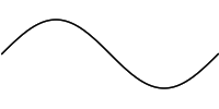
> sineWave = curve 0 (2 * pi) $ \t -> Vec t (sin t)

The section on rendering below explains how the points of the curve gets translated to pixels in the final image.

Combining images

Images form a monoid, so you can combine them using mappend (or the friendlier <>):

> cosineWave = curve 0 (2 * pi) $ \t -> Vec t (cos t)
> waves = sineWave <> cosineWave

It makes no difference for this example, but later it will be important to keep in mind that the left argument goes on top of the right argument. The chapter on blending looks at the various ways to combine images in more detail.

Extending curves

Two curves can be concatenated into a single curve using the +++ combinator.

> waves1 = sineWave +++ curve (2 * pi) (3 * pi) (\t -> Vec t (cos t))

If the end-points don't coincide, a straight line segment is added to connect the two 2. The combinators <++ and ++> adds a straight line segment to either end of a curve.

> waveBlock = botL <++ sineWave ++> botR ++> botL
>   where
>     botL = Vec 0 (-1.2)
>     botR = Vec (2 * pi) (-1.2)

Shape examples

With the tools introduced so far we can build some simple geometric figures. First, a circle 3:

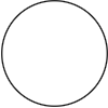
> unitCircle = curve 0 (2 * pi) $ \t -> Vec (cos t) (sin t)

Next, we'll reimplement the line and poly functions from the library:

> line' p q = curve_ $ \t -> diag (1 - t) * p + diag t * q
> poly' (p:q:ps) = foldl (++>) (line' p q) (ps ++ [p])

The curve_ lets you omit the start and end values for the parameter when they are 0 and 1. Interpolating between two points is sufficiently useful to warrant its own library function interpolate, so we can define line' more elegantly as

> line' p q = curve_ $ interpolate p q

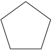
The poly function creates a closed 4 polygon from the given points so to create a box we just give the four corners.

> box w h = poly [0, Vec w 0, Vec w h, Vec 0 h]
> goldenBox = box ((1 + sqrt 5) / 2) 1

Regular n-sided polygons are also easy to define 5 using poly.

> regularCorners n =
>   [ Vec (cos x) (sin x)
>   | i <- [0..n - 1]
>   , let x = pi/2 + 2 * pi * fromIntegral i / fromIntegral n ]
>
> regularPoly = poly . regularCorners

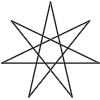
Reordering the vertices of an odd-sided regular polygon we can make a star:

> interleave []     ys = ys
> interleave (x:xs) ys = x : interleave ys xs
>
> regularStar n = poly $ uncurry interleave
>                      $ splitAt (div n 2 + 1) $ regularCorners n

Concatenating vs. combining

A natural question to ask is: what's the difference between using +++ and using <> on two curves with coinciding concatenation points? The non-answer is that in the first case you get an image with a single curve and the second case you get an image with two curves. This difference becomes most obvious once you start filling curves (see the chapter on curve styles) but we can observe it already with the tools we have.

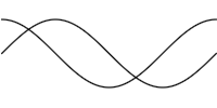
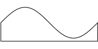
Let's define a reversed version of the sine wave, which starts at 2π and ends at 0, but consists of exactly the same points as the previous sine wave.

> sineWaveR = curve 0 (2 * pi) $ \t -> Vec (r t) (sin (r t))
>   where r t = 2 * pi - t

This is in fact a useful operation to have when concatenating curves, so it's defined in the library as reverseImage. Using this we can define

> sineWaveR = reverseImage sineWave

Now, let's look at the difference between combining and concatenating sineWave and sineWaveR.

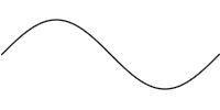
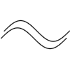
> combined     = sineWave <>  sineWaveR
> concatenated = sineWave +++ sineWaveR

combined

concatenated

If you look closely, you can see that the first image, which used <>, is darker and less smooth than the one using +++. Basically what happens is that in the combined case the sine wave is drawn twice, once for each curve, whereas each point on the concatenated curve is only drawn once, even though the curve passes through it twice. The section on rendering below explains the rendering process in more detail.

Transformations

It would be quite awkward to construct images just using curve and <>, so it make things easier there is a set of transformation combinators to transform images. The basic function is the transform function of the Transformable class:

> transform :: Transformable a => (Point -> Point) -> a -> a

Transforming an image applies the transformation function to all points of the curves of the image 6. For instance,

> twoWaves = sineWave <> transform (+ Vec 0.3 0.7) sineWave

For convenience a number of common transformations are defined in the library. Moving an image by a given vector, as above, can be done with the translate function, so twoWaves can be defined equivalently as

> twoWaves = sineWave <> translate (Vec 0.3 0.7) sineWave

The scale and rotate functions do what their names suggest:

> threeWaves = sineWave
>           <> scale 1.5 sineWave
>           <> rotate (pi/4) sineWave

Notice how both rotation and scaling are centered at the origin. The functions scaleFrom and rotateAround can be used to specify a different center.

> threeWaves' = sineWave
>            <> scaleFrom c 1.5 sineWave
>            <> rotateAround c (pi/4) sineWave
>   where c = Vec pi 0

The transformations above are all linear transformations, but any (continuous 7) function can be used to transform an image.

> wavyWave = transform (\p -> p + Vec 0 (cos (4 * getX p) / 2))
>                      sineWave

Rendering images

Although we've seen lots of example images, we haven't talked about how to get an actual picture from an Image. The function that does this is renderImage, which takes an image and writes it to a PNG file with the specified name. For instance

> saveBox :: IO ()
> saveBox = renderImage "box.png" 100 100 white
>         $ translate 10 (box 80 80)

creates the following 100x100 PNG file box.png:

Note how the points in the image correspond directly to pixels in the final picture. If we make the box wider it doesn't fit in the picture:

> saveBox' :: IO ()
> saveBox' = renderImage "box.png" 100 100 white
>          $ translate 10 (box 100 80)

In all the examples above we never cared about making sure that everything fit nicely in the final picture. In fact, if there had been a direct correspondence between points and pixels most examples above would only have been a few pixels wide. Indeed, having to worry about final pixel coordinates would be very tedious if all you want to do is create some nice figures. To deal with this there are two functions for automatically fitting an image inside some given bounds: autoFit and autoStretch.

> autoFit     :: Point -> Point -> Image -> Image
> autoStretch :: Point -> Point -> Image -> Image

Both functions take two points describing the bottom-left and top-right corners of a rectangle, and an image which is resized and moved to fit inside that rectangle. The difference between them is that autoFit preserves the aspect ratio of the image, whereas autoStretch scales the X and Y dimensions independently.

> fit     = autoFit     0 (Vec 200 100) unitCircle
> stretch = autoStretch 0 (Vec 200 100) unitCircle

autoFit

autoStretch

▲ 1 Note that Point is just a synonym for Vec, the type of 2-dimensional vectors.

▲ 2 To skip connecting the end-points, use +.+ instead.

▲ 3 There is a circle combinator in the library which takes the center and radius of the circle as parameters.

▲ 4 The lineStrip combinator is your friend if you don't want to close the polygon.

▲ 5 In fact, regularPoly is already defined in the Geometry module.

▲ 6 This isn't quite true, but true enough for our current purposes. See the chapter on advanced curves for more details.

▲ 7 Curve functions need to be continuous for the rendering algorithm to not get confused.